




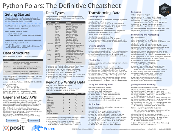
Polars is a library for transforming, analyzing, and visualizing data with a fast and expressive DataFrame API. It was first released by Ritchie Vink in 2020.
Install Polars with all of its optional dependencies from the terminal:
uv pip install "polars[all]"Import Polars in Python, and confirm which versions of Polars and its dependencies you have installed:
import polars as pl

pl.show_versions()
Polars queries typically read data, transform it, and write the result back out. A complete query is often a single chain of method calls:
fruit = pl.read_csv("fruit.csv")

fruit.filter(
    (pl.col("weight") > 1000) & pl.col("is_round")
).write_parquet("fruit.parquet")
Throughout this cheatsheet, df is a DataFrame, lf is a LazyFrame, o is a
second DataFrame to combine with df, and e stands for any expression.
So e.abs() means “call .abs() on an expression”, as in pl.col("x").abs().
Data Structures#
Polars stores all of its data in either a Series or a DataFrame.
| Structure | Description |
|---|---|
Series |
One-dimensional. Holds a sequence of values of the same data type. |
DataFrame |
Two-dimensional. Has rows and columns. One or more Series, all of the same length. |
LazyFrame |
Resembles a DataFrame but holds no data. A blueprint for generating a DataFrame. |
Unlike pandas, Polars DataFrames do not have a row index, and the API favors immutability and method chaining over in-place modifications.
-
Create a Series by passing a name and a sequence of values:
series = pl.Series("sales", [150.00, 300.00, 250.00]) -
Create a DataFrame from a dictionary of columns, where each value is a Series or a plain Python sequence. You can also use any of the
pl.read_*()functions to create one from a file:df = pl.DataFrame({ "sales": series, "id": [41, 42, 43] }) -
Because there is no row index, add one explicitly as a column when you need it:
df.with_row_index("id") -
Turn a DataFrame into a LazyFrame. Alternatively, start from a LazyFrame directly with any of the
pl.scan_*()functions:lf = df.lazy()
Eager and Lazy APIs#
The eager API executes immediately, whereas the lazy API builds an optimized query plan first. The optimizer automatically applies predicate pushdown (filtering as early as possible) and projection pushdown (dropping columns that are never used).
You move between the two representations with .lazy() and .collect(): .lazy()
turns a DataFrame into a LazyFrame, and .collect() executes a LazyFrame and gives
you a DataFrame back.
-
Turn a DataFrame into a LazyFrame, and execute a LazyFrame to get a DataFrame:
lf = df.lazy() df = lf.collect() -
Use the streaming engine to process data out-of-core, so that datasets larger than memory can still be handled:
lf.collect(engine="streaming") -
Print the optimized query plan as text, or visualize it as a graph, to see what the optimizer decided to do:
lf.explain() lf.show_graph() -
Execute the query and return per-node timings, which tells you where the time actually goes:
lf.profile()
Data Types#
Polars implements most of the Apache Arrow memory specification, which is an efficient columnar format for flat and hierarchical data.
| Group | Type | Notes |
|---|---|---|
| Numeric | Decimal |
128 bits, precision, scale |
Float32 |
Ranges ±3.4×10³⁸ | |
Float64 |
Ranges ±1.8×10³⁰⁸ | |
Int8 |
Ranges ±128 | |
Int16 |
Ranges ±32,768 | |
Int32 |
Ranges ±2.1×10⁹ | |
Int64 |
Ranges ±9.2×10¹⁸ | |
Int128 |
Ranges ±3.4×10³⁸ | |
UInt8 |
Ranges 0–255 | |
UInt16 |
Ranges 0–65,535 | |
UInt32 |
Ranges 0–4.3×10⁹ | |
UInt64 |
Ranges 0–1.8×10¹⁹ | |
| Temporal | Date |
Days since Unix epoch |
Datetime |
Microseconds since epoch | |
Duration |
Time duration / delta | |
Time |
Time of day | |
| Nested | Array |
Fixed-length sequence |
List |
Variable-length sequence | |
Struct |
Multiple fields with names | |
| String | String |
UTF-8 text, variable length |
Categorical |
Dict of Strings | |
Enum |
Fixed dict of Strings | |
| Other | Boolean |
True / False |
Binary |
Raw bytes | |
Null |
Represents Null / None |
Inspecting Types#
-
Get a dictionary of column names and data types, or just the list of data types:
df.schema df.dtypes -
Print one row per column, including data types, which is useful for wide DataFrames where printing the DataFrame itself is unreadable:
df.glimpse() -
Compute per-column summary statistics, including the number of nulls:
df.describe() -
Report the in-memory size of the DataFrame in the unit you ask for:
df.estimated_size("mb")
Casting#
-
Cast a column to another data type. By default the cast is strict, so a value that does not fit raises an error:
df.select(pl.col("id").cast(pl.UInt64)) -
Pass
strict=Falseto cast without raising. Values that overflow the target type become nulls instead:df.select(pl.col("id").cast(pl.Int8, strict=False))
Reading and Writing Data#
Polars has four families of input and output functions, and which one you want depends on whether you are working eagerly or lazily:
read_*()reads data into a DataFrame.scan_*()creates a LazyFrame, deferring the actual reading until you collect.write_*()writes a DataFrame to disk or to cloud storage.sink_*()streams data to disk or to cloud storage without holding it all in memory.
Not every format supports all four operations:
| Format | read |
scan |
write |
sink |
|---|---|---|---|---|
| Avro | ✓ | ✓ | ||
| Clipboard | ✓ | ✓ | ||
| CSV | ✓ | ✓ | ✓ | ✓ |
| Database | ✓ | ✓ | ||
| Delta Lake | ✓ | ✓ | ✓ | ✓ |
| Excel / ODS | ✓ | ✓ | ||
| Iceberg | ✓ | ✓ | ✓ | |
| IPC / Feather | ✓ | ✓ | ✓ | ✓ |
| JSON | ✓ | ✓ | ||
| NDJSON | ✓ | ✓ | ✓ | ✓ |
| Parquet | ✓ | ✓ | ✓ | ✓ |
| PyArrow Dataset | ✓ |
Keyword arguments that many of these functions accept include
schema_overrides, n_rows, row_index_name, storage_options, and
compression.
-
Scan files in cloud storage by passing a URI with a glob pattern, and use
storage_optionsto supply credentials and region settings:pl.scan_parquet( "s3://bucket/*.parquet", storage_options={"aws_region": "us-east-2"} ) -
Stream a query straight to a partitioned Parquet dataset, writing one directory per distinct value of the key column:
lf.sink_parquet(pl.PartitionBy("out/", key="x"))
Transforming Data#
Selecting Columns#
Keep columns based on their name, data type, or position.
-
Select columns by name:
df.select("a", "b") -
Select the result of an expression, so that you can transform columns on their way out:
df.select(pl.col("x") * 2) -
Give the result of an expression a name by using a keyword argument, which produces a new column:
df.select(doubled=pl.col("x") * 2) -
Select columns whose names match a regular expression. The pattern must start with
^and end with$:df.select(pl.col("^.*_color$")) -
Select every column:
df.select(pl.all())
Use column selectors for more flexibility.
They can be combined using the set operators |, &, -, ^, and ~.
-
Import the selectors module, then select columns by data type or by name pattern. See also
cs.string(),cs.contains(), andcs.first():import polars.selectors as cs df.select(cs.numeric()) df.select(cs.starts_with("val")) -
Drop columns instead of keeping them. Pass
strict=Falseso that names which do not exist are ignored rather than raising an error:df.drop("a", "y", strict=False)
Creating Columns#
New columns are added to the right of the existing ones.
-
Add a new column computed from an expression, naming it with a keyword argument:
df.with_columns(new=pl.col("a") + 1) -
Replace an existing column by producing an expression with the same name. Here, nulls in column
aare replaced with zeros:df.with_columns(pl.col("a").fill_null(0)) -
Add a column with the same literal value in every row:
df.with_columns(ones=pl.lit(1)) -
Add a column of row indices. Use
offsetto start counting somewhere other than zero:df.with_row_index(name="id", offset=1)
Filtering Rows#
Keep rows according to the values in one or more columns or expressions.
-
Filter on an existing boolean column by passing its name:
df.filter("valid") -
Filter with a single expression:
df.filter(pl.col("x") > 5) -
Pass multiple expressions to combine them with a logical AND. You can also write the AND explicitly with
&, in which case each comparison needs its own parentheses:df.filter(pl.col("valid"), pl.col("x") > 5) df.filter(pl.col("valid") & (pl.col("x") > 5)) -
Use
|for a logical OR:df.filter(pl.col("valid") | (pl.col("x") > 5)) -
Filter with keyword-argument constraints, which is shorthand for testing equality and combining the results with AND:
df.filter(valid=True, x=5) -
Keep only rows without any missing values, or restrict the check to specific columns:
df.drop_nulls() df.drop_nulls("x") -
Remove duplicate rows. Use
subsetto decide which columns define a duplicate, andkeepto choose which of the duplicates survives:df.unique(subset=["x"], keep="first")
Slicing and Sampling Rows#
Keep rows based on their position.
-
Keep the first rows, or the last rows. Both default to five:
df.head() df.tail(10) -
Keep a contiguous slice by giving an offset and a length. This keeps the third row through the seventh:
df.slice(2, 5) -
Keep every nth row:
df.gather_every(2) -
Take a random sample of rows. Use
with_replacement=Trueto allow the same row to be drawn more than once, orfractionto sample a proportion instead of a fixed number:df.sample(10) df.sample(10, with_replacement=True) df.sample(fraction=0.2)
Sorting Rows#
Reorder rows according to the values in one or more columns or expressions.
-
Sort by a single column, ascending by default, or by multiple columns in sequence:
df.sort("x") df.sort("x", "y") -
Move nulls to the end rather than the beginning:
df.sort("x", nulls_last=True) -
Reverse the order. When sorting by several columns, pass a list of booleans to set the direction per column:
df.sort("x", descending=True) df.sort("x", "y", descending=[False, True]) -
Sort by the result of an expression rather than by a column, such as a computed ratio or the length of a list:
df.sort(pl.col("x") / pl.col("y")) df.sort(pl.col("l").list.len()) -
Keep only the k largest or smallest rows according to a column, which is cheaper than sorting everything and then slicing:
df.top_k(5, by="score")
df.bottom_k(5, by="score")
Reshaping#
Go from wide to long and back again.
-
Make a DataFrame longer by turning the values of one or more columns into rows, keeping
indexcolumns as identifiers:df.unpivot(on=["c"], index="id") -
Make a DataFrame wider by turning the values of a column into new columns. If the combination of
onandindexis not unique, supply anaggregate_functionto decide how to combine the collisions:df.pivot(on="c", index="id", values="x") df.pivot(on="c", index="id", values="x", aggregate_function="sum") -
Expand a list column so that each element gets its own row, repeating the other columns:
df.explode("l") -
Expand a struct column so that each field becomes its own column:
df.unnest("s") -
Swap rows and columns. Use
include_header=Trueto keep the original column names as a column:df.transpose(include_header=True) -
Split a DataFrame into a list of smaller DataFrames, one per distinct value of the given column:
df.partition_by("group")
Summarizing and Aggregating#
Split. Apply. Combine.
-
Split a DataFrame into groups by one or more columns. This gives you a
GroupByobject that you then aggregate:dfg = df.group_by("x") dfg = df.group_by("x", "y") -
Apply a ready-made summary to every group. Count the rows per group, take the first rows of each group, or compute the mean of every column per group:
dfg.len() dfg.head(2) dfg.mean() -
Apply your own function to each group when no built-in aggregation fits:
dfg.map_groups(...) -
Use
agg()for full control over the aggregation. Passing an expression without an aggregating method collects the values into a list, and naming the result with a keyword argument gives the new column a sensible name:dfg.agg(...) dfg.agg(pl.col("y")) dfg.agg(avg=pl.col("y").mean()) -
Use a window expression with
over()to add an aggregation as a new column on the original DataFrame, without collapsing the rows:df.with_columns(avg=pl.col("y").mean().over("x")) -
Group by a time value or an index instead of by a category.
group_by_dynamic()creates windows of a fixed duration, andgroup_byadds a regular grouping on top:df.group_by_dynamic("timestamp", every="1h", group_by="store") -
Use
rolling()for a window that moves with every row rather than in fixed steps. This computes a seven-day rolling sum of sales per store:df.rolling(index_column="date", period="7d", group_by="store").agg( pl.col("sales").sum() ) -
Create the rows that are missing from a regular time series, so that every interval is represented:
df.upsample( time_column="date", every="1d", group_by="store", maintain_order=True ) -
Aggregate across columns rather than down them. The horizontal functions combine several columns within each row:
df.select(pl.sum_horizontal(cs.numeric()))
df.select(pl.any_horizontal(cs.boolean()))
Joining and Concatenating#
Combine multiple DataFrames into one.
-
Join two DataFrames on a shared key. The default is an inner join, which keeps only the rows that match on both sides:
df.join(o, on="key") -
Use
howto choose a different join strategy. A left join keeps every row ofdf:df.join(o, on="key", how="left") -
When the key has a different name in each DataFrame, name both sides explicitly:
df.join(o, left_on="a", right_on="b") -
A full outer join keeps all rows from both sides. Add
coalesce=Trueto merge the two key columns into one:df.join(o, on="key", how="full", coalesce=True) -
Filtering joins return columns from
dfonly, and useopurely as a filter. A semi join keeps the rows ofdfthat have a match, and an anti join keeps the rows that do not:df.join(o, on="key", how="semi") df.join(o, on="key", how="anti") -
A cross join produces the Cartesian product of both DataFrames and therefore needs no key:
df.join(o, how="cross") -
Join on the nearest match rather than an exact one, which is the usual way to line up two time series. Use
byto match exactly on some columns first:df.join_asof(o, on="ts", by="i") -
Join on an arbitrary predicate for inequality or other non-equi joins:
df.join_where(o, pl.col("a") >= pl.col("b"))
Common keyword arguments for df.join() are left_on, right_on, coalesce,
join_nulls, suffix, and validate, where validate accepts "m:m", "m:1",
"1:m", and "1:1".
-
Stack DataFrames on top of each other, which requires matching columns:
pl.concat([df, o]) -
Place DataFrames side by side instead, or take the union of their columns and fill in the gaps with nulls:
pl.concat([df, o], how="horizontal") pl.concat([df, o], how="diagonal") -
Use a relaxed strategy to coerce mismatched data types instead of raising an error:
pl.concat([df, o], how="vertical_relaxed") -
Update the values in
dfwith the non-null values from another DataFrame, matching rows on a key:df.update(o, on="id", how="left")
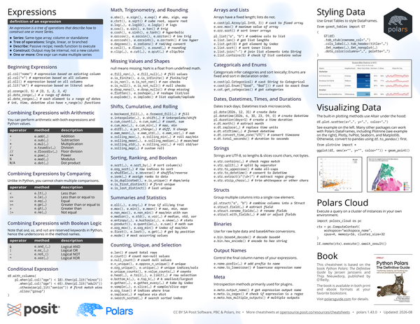
Expressions#
Definition of an expression
An expression is a tree of operations that describe how to construct one or more Series.
- Series: Same-type array; column or standalone
- Tree of operations: Single, linear, or branched
- Describe: Passive recipe; needs function to execute
- Construct: Output may be internal, not a new column
- One or more: One expression can make multiple Series
Beginning Expressions#
Every expression starts from a column, from all columns, or from a literal value.
-
Build an expression based on an existing column, on all columns, or on a literal value. Note that
pl.col("*")andpl.all()are equivalent:pl.col("name") pl.col("*") pl.all() pl.lit("ok") -
Generate a range of integers, where the stop value is exclusive. This produces
[0, 1, 2, 3, 4]:pl.arange(0, 5) -
Generate a range of dates. The singular form produces one range, while the plural form produces a column of ranges, one per row. Integers, times, and datetimes have their own
*_range()and*_ranges()functions:pl.date_range(...) pl.date_ranges(...)
Combining Expressions with Arithmetic#
You can perform arithmetic with both expressions and plain Python values. Every operator has an equivalent method, which is handy when you prefer to keep a chain of method calls unbroken.
| Operator | Method | Description |
|---|---|---|
+ |
e.add(...) |
Addition |
- |
e.sub(...) |
Subtraction |
* |
e.mul(...) |
Multiplication |
/ |
e.truediv(...) |
Division |
// |
e.floordiv(...) |
Floor division |
** |
e.pow(...) |
Power |
% |
e.mod(...) |
Modulus |
| N/A | e.dot(...) |
Dot product |
Combining Expressions by Comparing#
Unlike in Python, you cannot chain multiple comparisons.
Write (pl.col("x") > 0) & (pl.col("x") < 10) rather than 0 < pl.col("x") < 10.
| Operator | Method | Description |
|---|---|---|
< |
e.lt(...) |
Less than |
<= |
e.le(...) |
Less than or equal to |
== |
e.eq(...) |
Equal |
>= |
e.ge(...) |
Greater than or equal to |
> |
e.gt(...) |
Greater than |
!= |
e.ne(...) |
Not equal |
Combining Expressions with Boolean Logic#
Note that and, or, and not are reserved keywords in Python, hence the
underscores in the method names.
| Operator | Method | Description |
|---|---|---|
& |
e.and_(...) |
Logical AND |
| |
e.or_(...) |
Logical OR |
~ |
e.not_() |
Logical NOT |
^ |
e.xor(...) |
Logical XOR |
Conditional Expression#
Chain when() and then() to build a conditional expression, and close it with
otherwise().
Conditions are evaluated in order and the first match wins, so put the most
specific condition first:
df.with_columns(
    pl.when(pl.col("age") < 18).then(pl.lit("minor"))
      .when(pl.col("age") < 65).then(pl.lit("adult"))
      .otherwise(pl.lit("senior"))
      .alias("group")
)
Math, Trigonometry, and Rounding#
e.abs(),e.sign(),e.exp(): absolute value, sign, and exponential.e.cbrt(),e.sqrt(): cube root and square root.e.log(...),e.log10(),e.log1p(): logarithms.e.cos(),e.sin(),e.tan(): trigonometric functions.e.cosh(),e.sinh(),e.tanh(): hyperbolic functions.e.arccos(),e.arcsin(),e.arctan(): inverse trigonometric functions.e.arccosh(),e.arcsinh(),e.arctanh(): inverse hyperbolic functions.e.degrees(),e.radians(): convert between radians and degrees.e.ceil(),e.floor(),e.round(...): rounding.e.clip(...),e.cut(...),e.qcut(...): clip values to a range, or bin them into intervals of your choosing or into quantiles.
Missing Values and Shapes#
In Polars, null means missing, whereas NaN is a float that results from
undefined math such as 0 / 0.
The two are handled by separate methods.
e.fill_nan(...),e.fill_null(...): fill missing values.e.is_finite(),e.is_infinite(): check for finite and infinite values.e.is_nan(),e.is_not_nan(): check for NaN.e.is_null(),e.is_not_null(): check for null.e.drop_nans(),e.drop_nulls(): drop missing values.e.flatten(),e.reshape(...): reshape a list or column.e.explode(),e.implode(): turn a list into rows, or gather rows into a list.
Shifts, Cumulative, and Rolling#
e.backward_fill(...),e.forward_fill(...): fill nulls from the next or the previous value.e.interpolate(...),e.shift(...): interpolate between known values, or move values up or down.e.cum_count(...),e.cum_sum(...): cumulative count and sum.e.cum_max(...),e.cum_min(...): cumulative maximum and minimum.e.diff(...),e.pct_change(...): difference and percentage change between rows.e.ewm_mean(...),e.ewm_std(...),e.ewm_var(...): exponentially weighted moving statistics.e.rolling_max(...),e.rolling_min(...): rolling maximum and minimum.e.rolling_mean(...),e.rolling_median(...): rolling mean and median.e.rolling_std(...),e.rolling_var(...): rolling standard deviation and variance.e.rolling_map(...): apply your own function over a rolling window.
Sorting, Ranking, and Boolean#
e.sort(...),e.sort_by(...): sort a column by its own values, or by the values of other columns.e.arg_sort(...): return the row indices that would sort the column.e.shuffle(...),e.reverse(): shuffle values randomly, or reverse their order.e.rank(...): assign ranks to the data.e.is_duplicated(),e.is_unique(): mark which values are duplicated and which are unique.e.is_first_distinct(),e.is_last_distinct(): mark the first or the last occurrence of each distinct value.
Summaries and Statistics#
e.all(...),e.any(...): true if all or any of the values are true.e.max(),e.min(),e.mean(): maximum, minimum, and mean.e.nan_max(),e.nan_min(): maximum and minimum that propagate NaN.e.median(),e.std(),e.var(...): median, standard deviation, and variance.e.entropy(...),e.kurtosis(...),e.skew(...): distribution statistics.e.product(),e.quantile(...),e.sum(): product, quantile, and sum.e.arg_max(),e.arg_min(): index of the maximum and minimum value.e.first(),e.last(),e.get(...): get a value by position.e.mode(): the most frequently occurring values.
Counting, Unique, and Selection#
e.len(): count all rows, including nulls.e.count(): count only the non-null values.e.null_count(): count the null values.e.n_unique(),e.approx_n_unique(): number of unique values, exactly or approximately.e.arg_unique(),e.unique(...): indices of the unique values, or the unique values themselves.e.unique_counts(),e.value_counts(...): how often each unique value occurs.e.head(...),e.tail(...),e.limit(...): select rows from the start or the end.e.bottom_k(...),e.top_k(...): the k smallest or largest values.e.gather(...),e.gather_every(...): take values by index, or take every nth value.e.sample(...),e.slice(...): sample or slice within an expression.e.arg_true(): the indices where the value is true.e.replace(...): replace values using a dictionary.e.search_sorted(...): find the insertion index in a sorted column.
Arrays and Lists#
Arrays have a fixed length; lists do not.
Array methods live under the arr namespace and list methods under list.
-
Cast a column to an array of a fixed length, then use the array namespace:
e.cast(pl.Array(pl.Int8, 3)) e.arr.max() e.arr.sort() -
Combine several columns into a single list column:
pl.list("a", "b") -
Work with the contents of a list column: get the length of each list, get an element by index, sort the elements within each list, join them into a single string, or test whether a value is present:
e.list.len()
e.list.get(0)
e.list.sort()
e.list.join("-")
e.list.contains(5)
Categoricals and Enums#
Categoricals infer their categories from the data and sort lexically, whereas Enums are fixed up front and sort in declaration order.
-
Cast a String column to a Categorical, or to an Enum with an exact set of allowed values:
e.cast(pl.Categorical) e.cast(pl.Enum(["Good", "Bad"])) -
Retrieve the categories that a Categorical column ended up with:
e.cat.get_categories()
Dates, Datetimes, Times, and Durations#
Dates track days, whereas Datetimes track microseconds.
Methods for working with them live under the dt namespace.
-
Construct a Date, a Datetime, or a Duration from their components:
pl.date(2026, 12, 31) pl.datetime(2026, 6, 30, 23, 59, 0) pl.duration(days=1) -
Extract a single component, such as the month:
e.dt.month() -
Replace individual time units, leaving the rest untouched:
e.dt.replace(...) -
Format a datetime as a string using a format specification:
e.dt.strftime(...) -
Convert a datetime to another time zone:
e.dt.convert_time_zone("UTC") -
Express a duration as a number of seconds:
e.dt.total_seconds()
Strings#
Strings are UTF-8, so lengths and slices count characters, not bytes.
String methods live under the str namespace.
e.str.contains(...): check whether each value matches a regular expression.e.str.split(...): split each value by a separator into a list.e.str.to_uppercase(): make each value all-caps.e.str.to_datetime(): parse each value into a Datetime.e.str.extract(r"(\d+)"): extract the first regular expression capture group.e.str.strip_chars(...): trim whitespace, or other characters you specify, from both ends.
Structs#
A struct groups multiple columns into a single row element.
Struct methods live under the struct namespace.
-
Combine columns into a Struct, then extract a single field back out:
pl.struct("a", "b") e.struct.field(...) -
Rename the fields of a Struct, or add and adjust fields:
e.struct.rename_fields(...)
e.struct.with_fields(...)
Binaries#
Use the bin namespace for raw byte data and for base64 and hexadecimal
conversions.
-
Decode a base64 string, or encode bytes as a hexadecimal string:
e.bin.base64_decode()
e.bin.hex_encode()
Output Names#
Control the final column names of your expressions with the name namespace.
-
Add a prefix to the existing name, or lowercase it:
e.name.prefix(...)
e.name.to_lowercase()
Meta#
Introspection methods, primarily used when writing plugins, live under the meta
namespace.
e.meta.output_name(): get the name the expression will output.e.meta.is_regex(): check whether the expression is a regular expression.e.meta.has_multiple_outputs(): check whether the expression produces multiple outputs.
Styling Data#
Use Great Tables to turn a DataFrame
into a presentation-ready table.
Start from GT(df) and chain the methods that set up the stub and header, format
the values, and add color:
from great_tables import GT

(
    GT(df)
    .tab_stub(rowname_col="...")
    .cols_label(...)
    .tab_header(title="...")
    .fmt_number(...)
    .fmt_nanoplot(...)
    .data_color(columns="...", palette="...")
)
Visualizing Data#
The built-in plotting methods use Altair under the hood, and are available from the
plot namespace:
df.plot.scatter(x="...", y="...", color="...")
Many other packages can work with Polars DataFrames directly, including
Plotnine, Plotly, hvPlot, Seaborn, and Matplotlib.
For anything that cannot, convert to pandas first with df.to_pandas().
from plotnine import *

ggplot(df, aes(x="", y="", color="")) + geom_point()
Polars Cloud#
Execute a query on a cluster of instances in your own environment.
Describe the compute you want with a ComputeContext, then run a LazyFrame
remotely against it:
import polars_cloud as pc

ctx = pc.ComputeContext(
    workspace="workspace_name",
    cpus=4,
    memory=16,
    cluster_size=32
)

lf.remote(ctx).execute().await_result()Book#
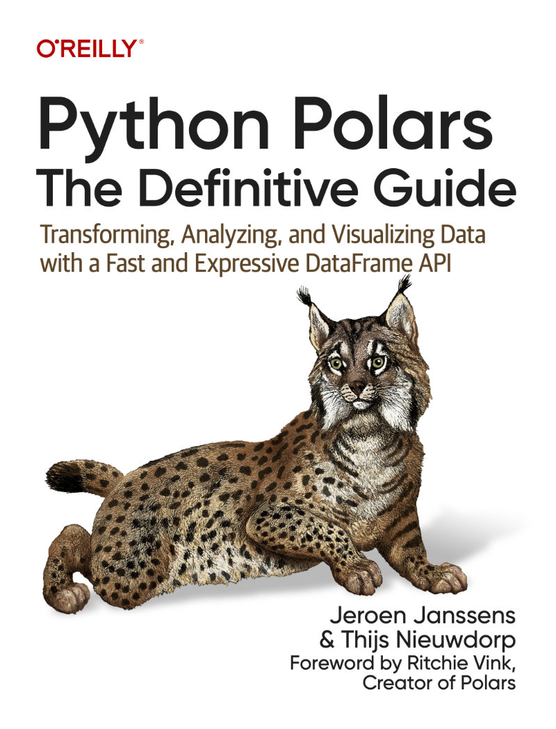 This cheatsheet is based on the book Python Polars: The Definitive Guide by
Jeroen Janssens and Thijs Nieuwdorp, published by O’Reilly.
The book is available in both print and ebook formats at your favorite bookstore.
Visit polarsguide.com for details.
This cheatsheet is based on the book Python Polars: The Definitive Guide by
Jeroen Janssens and Thijs Nieuwdorp, published by O’Reilly.
The book is available in both print and ebook formats at your favorite bookstore.
Visit polarsguide.com for details.


